The power of diversification and its limits by the example of DAX

Summary

• Sometimes (esp. to fool inexperienced retail investors) the diversification is claimed to be a silver bullet (even in a financial crisis).  I show that in crises the diversification effect weakens significantly but still persists (esp. for "defensive" stocks).
• I argue that in a normal (non-turbulent) market the diversification is very helpful in theory but also critically consider its applicability in practice.
• The results that we obtained for the DAX / German stock market should be extrapolated with caution for other markets. You will also see why it is better to watch and know the market (rather than to blindly rely on quantitative analysis and common sense).

In my previous critical post about the RoboAdvisors I mentioned that in a financial crisis the correlations between the assets grow (if panic breaks out they fall together) and the diversification reaches it its limit. However, in a discussion on NP they affirmed, the (conditional) correlations grow with volatility per se (i.e. not only with the "downside" volatility). Who is right?! The only way to check is to look at historical data, since without data you're just another person with an opinion (W. Edwards Deming). Still, dealing with real data there is a lot of subjective empiricism. Thus you should consider the data-driven conclusions also critically (and thus I provide you with source code and data: to make the results reproducible and to avoid Reinhart and Rogoff Excel error.

First of all what do we take as the German market proxy? Taking DAX is common but this is not the only option (in particular there is a very strong medium segment in Germany, so considering mDAX too would also be a good option). But for simplicity we stick to the DAX. However, there is another nuance: the 30 DAX stocks in 2007 and in 2016 are not the same (though, fortunately, most of them are). Again for simplicity we consider the DAX components as in 2016 and then loop them back. But e.g. Vonovia SE (VNA.DE) went public only on 11.07.2013, so there is no historical data for the loopback period before this date. Moreover, there are a lot of missing data for ProSieben and Volkwagen  (PSM.DE and VOW3.DE). Why? Well, because Yahoo.Finance, where we download the data from, is not perfect! The quick (and no so dirty) way is just to throw away VNA, PSM and VOW3. These are just 3 of 30 stocks, so they should not mean much. Moreover, it is in either case good to remove Volkswagen (or to consider it in a special way) because in 2008 there was a short squeeze as Porsche tried to acquire Volkwagen and recently in September 2015 the Dieselgate occured. Hadn't we know the history (and relied only on math) we would confront a misleading anomaly! Thus I am usually pretty skeptical about purely quantitative strategies that rely on huge data sets from deep past.

Further, what is an extraordinary volatility?! Since I daily watch the DAX for more than 10 years, I said (before I plotted the Figure 1) the DAX is extraordinary volatile when the daily returns exceed ±3%.

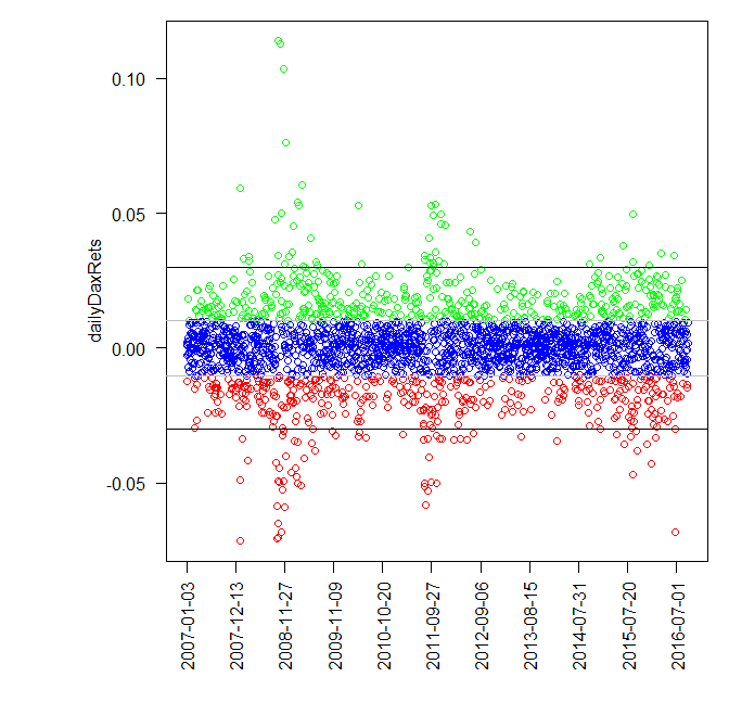
On the other hand if we apply a straightforward k-means clustering (which is likely the most frequently used but not necessarily the best) clustering approach, the frontier of "normal" and "extraordinary" lies at approximately ±1%, which is also conform to my practical experience. Still I choose the ±3% threshold since we see that these returns are accumulated around financial crisis in 2008, US sovereign rating downgrade in 2011, significant DAX correction after the exuberant growth in 2015 and the last red one in 2016 is Brexit.

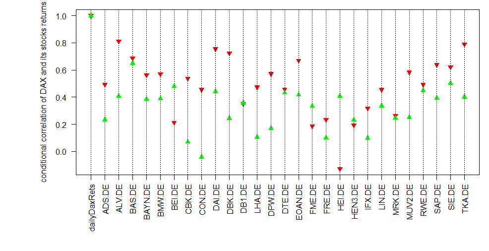
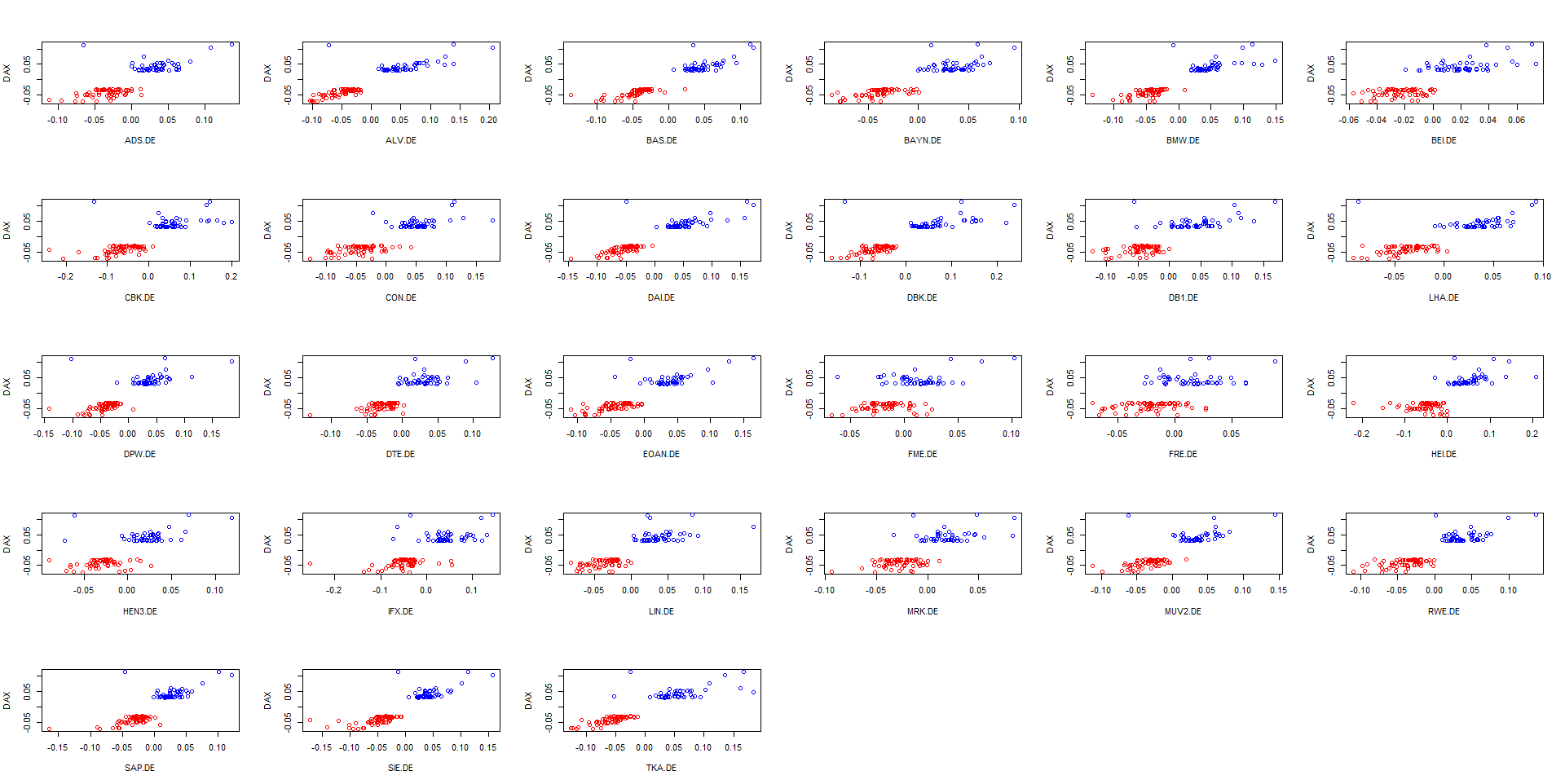
Calculating the correlations of stock daily returns with DAX daily returns, conditioned on the latter (green when DAX grows more than 3%, red when it falls more than -3% per day) we see that the conditional correlations do differ! When the market (in our analysis proxied by the DAX) falls, most of stocks tend to correlate stronger with the DAX! So, from formal point of view we have shown that in the (extremely) bear market the diversification effect is weaker. It is also confirmed by Figure 3, which shows us that some stock did fall when the DAX grew extremely but no stock has ever grown as DAX fall more than -3%.

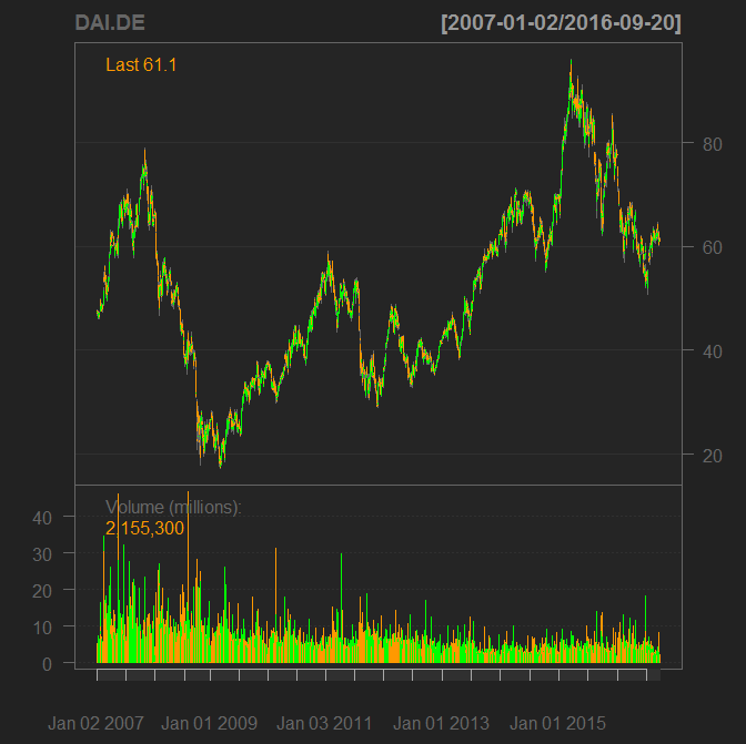
The first idea might be to choose the stocks for which the green triangle lies over the red. It is even backed by the common sense: whether crisis or not, there will be demand for the production of pharma companies like Fresenius (FME.DE und FRE.DE) and Beiersdorf (BEI.DE) as well as for consumer chemical goods Henkel (HEI.DE). Analogously the automotive (DAI.DE and BMW.DE) will likely fall in any crisis, since a new car is the last what is bought when things go bad. Also the Lufthansa (LHA.DE) is likely affected by crises since both leisure and business traveling shrinks.

However, we should avoid messing with the cause and the effect. For instance, the bank stocks (CBK.DE and DBK.DE) fell in crisis not because they generally do but first of all because the crisis in 2008 was the bank crisis. Moreover, why the utility companies E.ON and RWE (EOAN.DE and RWE.DE) did fall, although the common sense says the utility stocks are a safe harbor in crisis. Generally yes, but in Germany not anymore. RWE and E.ON were too retroactive and missed the colossal transformation to the renewable energy, which was followed by the liberalization of the energy market. And Fukushima meltdown was the final knock-out strike for RWE and E.ON since they had to shut down their nuclear power plants. Essentially, they are doomed and the shareholders get especially nervous everytime as the market declines.
Last but not least, the correlation values of HeidelbergCement (HEI.DE) are also somewhat misleading. In 2008 it fell as strong as the bank stocks since it was a bank and real estate crisis. However, as the market realized that zero interest rates are to persist for a long time, the Germans massively started getting mortgages. So nowadays the real estate branch booms in Germany, thus HEI.DE has such conditional correlations. Still I would not hold it as a defensive stock since I am quite sure the German real estate bubble will burst!
And of course even though HEI.DE negatively correlates with DAX when the latter extremely falls, it no way means that HEI.DE ever grew by these times (recall Figure 3). It simply means that (within the considered loopback period) HEI.DE on average fell less during turbulent times than DAX itself. But once again: in crisis they all fall: some more, some less but still they fall together! Thus don't believe those who affirm the diversification is a panacea.

On the other hand you also should not underestimate the diversification during a calm market regime. Finally a stock index like DAX (or better to say an ETF on it) is a (relatively broadly) diversified portfolio. One may tend to select only "the most promising" stocks, like e.g. German automotive stocks nowadays.

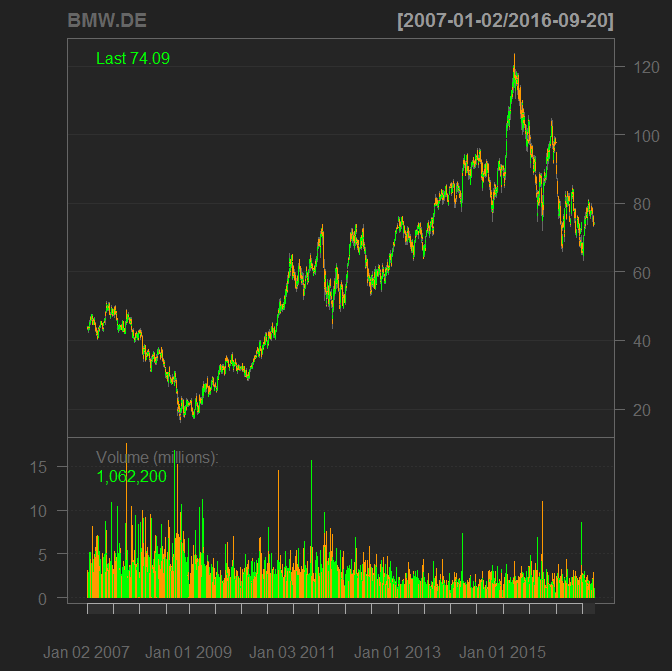
Figure 4 (click to enlarge): Daily charts of BMW and Daimler

Indeed, both Daimler and BMW are promising from technical and fundamental points of view (in particular, their P/E coefficients are about 7.5). But this "opportunity" persists for a long time and this is not an accident. First of all I already mentioned that new cars are hardly bought in crisis ⇒ risk! Secondly, the market is likely afraid of the Dieselgate. And last but not least, I personally would never consider Daimler for a long-term investment due to extreme arrogance, cultivated in their corporate culture. From their arrogance they tend to ignorance and will likely be unable to compete with Tesla and Google Car (Apple allegedly also runs a car project and, moreover, has lured the best young engineers from Daimler and BMW). And this is not new, recall the history of Ford if you doubt!

I also refer you to my book "Knowledge rather than Hope". In Chapter 5 I consider a portfolio of 10 assets with good odds about 13:5 and correlation coefficients about 0.2. The simulation gives us very promising future scenarios, which are much better than in case of the portfolio with the same odds but without a diversification. The nuance is that it is pretty hard to find ten good trading opportunities that are so loosely correlated :).

#uncomment if you don't have yet installed quantmod, sqldf and plyr packages
#install.packages("quantmod")
#install.packages("sqldf")
 
library(quantmod)
library(sqldf)

tickersDAX = c("ADS.DE", "ALV.DE", "BAS.DE", "BAYN.DE", "BMW.DE", "BEI.DE",
 "CBK.DE", "CON.DE", "DAI.DE", "DBK.DE", "DB1.DE", "LHA.DE",
 "DPW.DE", "DTE.DE", "EOAN.DE","FME.DE", "FRE.DE", "HEI.DE",
 "HEN3.DE","IFX.DE", "LIN.DE", "MRK.DE", "MUV2.DE","PSM.DE",
 "RWE.DE", "SAP.DE", "SIE.DE", "TKA.DE", "VOW3.DE","VNA.DE")
#load data from Yahoo.Finance
startDate = '2007-01-02'
endDate = '2016-09-20'

#get DAX componets (from/to are fixed for reproducibility)
getSymbols(tickersDAX, from=startDate, to=endDate)
#get DAX daily OHLC data from yahoo.finance 
getSymbols("^GDAXI", from=startDate, to=endDate)

#~ If you work with saved R workspace, copy and paste code starting from here ~#
#~ But don't forget library(quantmod) and library(sqldf) ~#

dailyDaxRets = as.numeric(ClCl(GDAXI))
elemsToTake = which(!is.na(dailyDaxRets)) #remove 1st "n/a" element
dailyDaxRets = dailyDaxRets[elemsToTake]
datesToTake = (index(GDAXI))[elemsToTake] 
kmClust = kmeans(dailyDaxRets, centers=3) #higly positive, normal and highly negative returns
colorz = c("green", "red", "blue" )
par(las=2)
par(mar=c(8,8,1,1))
plot(dailyDaxRets, col = colorz[kmClust$cluster], xaxt="n", xlab="")
labelz = seq(1, length(datesToTake), 242)
axis(side=1, at=labelz, labels=datesToTake[labelz])
middleDaxRets = dailyDaxRets[which(kmClust$cluster == 3)]
abline(h = min(middleDaxRets), col="grey" ) #approximately +/-1%
abline(h = max(middleDaxRets), col="grey" )
#my experience says the normal returns are between +/-3%, decide yourself for it or for k-means
abline(h=-0.03)
abline(h=0.03)


N_DAYS = length(datesToTake)
mainFrame = data.frame(datesToTake, dailyDaxRets)
N_TICKERS = length(tickersDAX) #30
for( i in 1:N_TICKERS)
{
 stock = eval(parse(text=tickersDAX[i]))
 stockRets = as.numeric(ClCl(stock))
 stockDates = index(stock)
 stockFrame = data.frame(stockDates, stockRets)
 mainFrame = sqldf("SELECT * FROM mainFrame LEFT JOIN stockFrame ON mainFrame.datesToTake = stockFrame.stockDates")
 mainFrame$stockDates <- NULL #remove temporarily column
 names(mainFrame)[names(mainFrame)=="stockRets"] <- tickersDAX[i] #rename to avoid dup-names } threshold = 0.03 superFrame = sqldf(paste("SELECT * FROM mainFrame WHERE dailyDaxRets>", threshold, sep=""))
superFrame$PSM.DE <- NULL
superFrame$VOW3.DE <- NULL
superFrame$VNA.DE <- NULL
superFrame$datesToTake <- NULL
superCor = round(cor(superFrame), 3)

subFrame = sqldf(paste("SELECT * FROM mainFrame WHERE dailyDaxRets<", -threshold, sep=""))
subFrame$PSM.DE <- NULL
subFrame$VOW3.DE <- NULL
subFrame$VNA.DE <- NULL
subFrame$datesToTake <- NULL
subCor = round(cor(subFrame), 3)

#plot figure 2
par(las=2)
par(mar=c(8,8,1,1))
labelz2 = names(subCor[,1])
plot(subCor[,1], col="red", pch=25, bg="red", xaxt="n", xlab="", ylab="conditional correlation of DAX and its stocks returns")
points( superCor[,1], col="green", pch=24, bg="green")
labelz2 = names(subCor[,1])
axis(side=1, at=seq(1:28), labels=labelz2)
abline(v=seq(1:28), lty=3)

#plot figure 3
par(mfrow=c(5,6))
d = (dim(subFrame))[2] #28, since we removed PSM, VOW3 and VNA
yLim = c(min(subFrame[, 1]), max(superFrame[, 1]))
for(i in 2:d)
{
 xLim = c(min(subFrame[, i]), max(superFrame[, i]))
 plot(subFrame[, i], subFrame[, 1], col="red", xlim=xLim, ylim=yLim, xlab=names(subFrame)[i], ylab="DAX")
 points(superFrame[, i], superFrame[, 1], col="blue")
}

R Workspace - use it you cannot get data from Yahoo.Finance or if these data are implausible